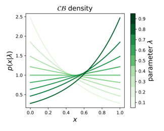
Continuous Bernoulli distribution

Continuous Bernoulli distribution

Probability density function
Notation	${\displaystyle {\mathcal {CB}}(\lambda )}$
Parameters	${\displaystyle \lambda \in (0,1)}$
Support	${\displaystyle x\in [0,1]}$
PDF	${\displaystyle C(\lambda )\lambda ^{x}(1-\lambda )^{1-x}\!}$ where ${\displaystyle C(\lambda )={\begin{cases}2&{\text{if }}\lambda ={\frac {1}{2}}\\{\frac {2\tanh ^{-1}(1-2\lambda )}{1-2\lambda }}&{\text{ otherwise}}\end{cases}}}$
CDF	${\displaystyle {\begin{cases}x&{\text{ if }}\lambda ={\frac {1}{2}}\\{\frac {\lambda ^{x}(1-\lambda )^{1-x}+\lambda -1}{2\lambda -1}}&{\text{ otherwise}}\end{cases}}\!}$
Mean	${\displaystyle \operatorname {E} [X]={\begin{cases}{\frac {1}{2}}&{\text{ if }}\lambda ={\frac {1}{2}}\\{\frac {\lambda }{2\lambda -1}}+{\frac {1}{2\tanh ^{-1}(1-2\lambda )}}&{\text{ otherwise}}\end{cases}}\!}$
Variance	${\displaystyle \operatorname {var} [X]={\begin{cases}{\frac {1}{12}}&{\text{ if }}\lambda ={\frac {1}{2}}\\-{\frac {(1-\lambda )\lambda }{(1-2\lambda )^{2}}}+{\frac {1}{(2\tanh ^{-1}(1-2\lambda ))^{2}}}&{\text{ otherwise}}\end{cases}}\!}$

In probability theory, statistics, and machine learning, the continuous Bernoulli distribution^[1][2][3] is a family of continuous probability distributions parameterized by a single shape parameter ${\displaystyle \lambda \in (0,1)}$, defined on the unit interval ${\displaystyle x\in [0,1]}$, by:

${\displaystyle p(x|\lambda )\propto \lambda ^{x}(1-\lambda )^{1-x}.}$

The continuous Bernoulli distribution arises in deep learning and computer vision, specifically in the context of variational autoencoders,^[4][5] for modeling the pixel intensities of natural images. As such, it defines a proper probabilistic counterpart for the commonly used binary cross entropy loss, which is often applied to continuous, ${\displaystyle [0,1]}$-valued data.^[6][7][8][9] This practice amounts to ignoring the normalizing constant of the continuous Bernoulli distribution, since the binary cross entropy loss only defines a true log-likelihood for discrete, ${\displaystyle \{0,1\}}$-valued data.

The continuous Bernoulli also defines an exponential family of distributions. Writing ${\displaystyle \eta =\log \left(\lambda /(1-\lambda )\right)}$ for the natural parameter, the density can be rewritten in canonical form: ${\displaystyle p(x|\eta )\propto \exp(\eta x)}$.

Related distributions

Bernoulli distribution

The continuous Bernoulli can be thought of as a continuous relaxation of the Bernoulli distribution, which is defined on the discrete set ${\displaystyle \{0,1\}}$ by the probability mass function:

${\displaystyle p(x)=p^{x}(1-p)^{1-x},}$

where ${\displaystyle p}$ is a scalar parameter between 0 and 1. Applying this same functional form on the continuous interval ${\displaystyle [0,1]}$ results in the continuous Bernoulli probability density function, up to a normalizing constant.

Beta distribution

The Beta distribution has the density function:

${\displaystyle p(x)\propto x^{\alpha -1}(1-x)^{\beta -1},}$

which can be re-written as:

${\displaystyle p(x)\propto x_{1}^{\alpha _{1}-1}x_{2}^{\alpha _{2}-1},}$

where ${\displaystyle \alpha _{1},\alpha _{2}}$ are positive scalar parameters, and ${\displaystyle (x_{1},x_{2})}$ represents an arbitrary point inside the 1-simplex, ${\displaystyle \Delta ^{1}=\{(x_{1},x_{2}):x_{1}>0,x_{2}>0,x_{1}+x_{2}=1\}}$. Switching the role of the parameter and the argument in this density function, we obtain:

${\displaystyle p(x)\propto \alpha _{1}^{x_{1}}\alpha _{2}^{x_{2}}.}$

This family is only identifiable up to the linear constraint ${\displaystyle \alpha _{1}+\alpha _{2}=1}$, whence we obtain:

${\displaystyle p(x)\propto \lambda ^{x_{1}}(1-\lambda )^{x_{2}},}$

corresponding exactly to the continuous Bernoulli density.

Exponential distribution

An exponential distribution restricted to the unit interval is equivalent to a continuous Bernoulli distribution with appropriate^[which?] parameter.

Continuous categorical distribution

The multivariate generalization of the continuous Bernoulli is called the continuous-categorical.^[10]

References

- ^ Loaiza-Ganem, G., & Cunningham, J. P. (2019). The continuous Bernoulli: fixing a pervasive error in variational autoencoders. In Advances in Neural Information Processing Systems (pp. 13266-13276).
- ^ PyTorch Distributions. https://pytorch.org/docs/stable/distributions.html#continuousbernoulli
- ^ Tensorflow Probability. https://www.tensorflow.org/probability/api_docs/python/tfp/edward2/ContinuousBernoulli Archived 2020-11-25 at the Wayback Machine
- ^ Kingma, D. P., & Welling, M. (2013). Auto-encoding variational bayes. arXiv preprint arXiv:1312.6114.
- ^ Kingma, D. P., & Welling, M. (2014, April). Stochastic gradient VB and the variational auto-encoder. In Second International Conference on Learning Representations, ICLR (Vol. 19).
- ^ Larsen, A. B. L., Sønderby, S. K., Larochelle, H., & Winther, O. (2016, June). Autoencoding beyond pixels using a learned similarity metric. In International conference on machine learning (pp. 1558-1566).
- ^ Jiang, Z., Zheng, Y., Tan, H., Tang, B., & Zhou, H. (2017, August). Variational deep embedding: an unsupervised and generative approach to clustering. In Proceedings of the 26th International Joint Conference on Artificial Intelligence (pp. 1965-1972).
- ^ PyTorch VAE tutorial: https://github.com/pytorch/examples/tree/master/vae.
- ^ Keras VAE tutorial: https://blog.keras.io/building-autoencoders-in-keras.html.
- ^ Gordon-Rodriguez, E., Loaiza-Ganem, G., & Cunningham, J. P. (2020). The continuous categorical: a novel simplex-valued exponential family. In 36th International Conference on Machine Learning, ICML 2020. International Machine Learning Society (IMLS).